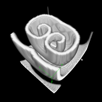
3D Reaction-Diffusion: Excitable Media

Persistent Identifier

Use this permanent link to cite or share this Morpheus model:

Introduction

This example uses the Barkley model of excitable media, similar to the Fitzhugh-Nagumo model to show how to model and visualize reaction-diffusion models in 3D.

Scroll wave appears in Barkley model of excitable media in 3D.

Description

This model defines a 3D cubic Lattice with noflux BoundaryConditions. Two Layers are defined for the two species: $u$ is the signal, and $v$ the refractoriness. As in the examples above, the DiffEqn as specified in the System in PDE. Nothing strange here.

To visualize the resulting scrolling waves in 3D, the TiffPlotter is used. This Analysis plugin writes TIFF image stacks that can be opened by image analysis software such as Fiji ImageJ. To import Morpheus TIFF images into Fiji, macro scripts are available that help you to create 3D ($xyz$), 4D ($xyzt$) or even 5D ($xyzct$) images and movies of your simulations.

Although unable to plot 3D, the GnuPlotter can still be helpful to plot a 2D slice. See Analysis/Gnuplotter/PDE/slice.

Things to try

Import resulting sequence of TIFF images in ImageJ or Fiji, and create 4D movie using ImageJ’s 3D plugin:
- Open u_v.tif in ImageJ: File → Open.
- Create hyperstack: Image → Hyperstack → Convert to Hyperstack. Channels ($c$): 2, Slices ($z$): 50, Frames ($t$): 51, Display Mode: Composite.
- Display in 4D: Plugins → 3D Viewer. Use default parameters. Press OK.

Reference

D. Barkley: A model for fast computer simulation of waves in excitable media. Physica 49D, 61–70, 1991.

Model

Get this model via:

Morpheus-Link or

Morpheus GUI: Examples → PDE → ExcitableMedium_3D.xml or

Download: ExcitableMedium_3D.xml

XML Preview

<MorpheusModel version="3">
    <Description>
        <Title>Example-ExcitableMedium-3D</Title>
        <Details>Simulates the Barkley model of an excitable medium, see: http://www.scholarpedia.org/article/Barkley_model
Derived from FitzHugh-Nagumo model and Hogdkin-Huxley model.

TIFF images can be viewed with external tools such as Fiji / ImageJ (http://fiji.sc/Fiji) or BioView3D (http://www.dimin.net/software/bioview3d/). The latter also reads the OME header for 3D,4D and 5D images.
 </Details>
    </Description>
    <Global>
        <Field symbol="u" value="if( l.x>=s.x/2-5 and l.x&lt;=s.x/2+5 and l.z>=s.z/2-5 and l.z&lt;=s.z/2+5 and l.y&lt;=s.y/4 , 1, 0 )">
            <Diffusion rate="0.5"/>
        </Field>
        <Field symbol="v" value="if(l.x&lt;=s.x/2 and l.z&lt;=(3*s.z)/4, 1, 0)">
            <Diffusion rate="0.5"/>
        </Field>
        <System solver="runge-kutta" time-step="0.05">
            <DiffEqn symbol-ref="u">
                <Expression>(1/e)*u*(1-u)*(u-((v+b)/a))</Expression>
            </DiffEqn>
            <DiffEqn symbol-ref="v">
                <Expression>u-v</Expression>
            </DiffEqn>
            <Constant symbol="e" value="0.02"/>
            <Constant symbol="a" value="0.8"/>
            <Constant symbol="b" value="0.01"/>
        </System>
    </Global>
    <Space>
        <Lattice class="cubic">
            <Size symbol="s" value="50 50 50"/>
            <BoundaryConditions>
                <Condition boundary="x" type="noflux"/>
                <Condition boundary="y" type="noflux"/>
                <Condition boundary="z" type="noflux"/>
                <Condition boundary="-x" type="noflux"/>
                <Condition boundary="-y" type="noflux"/>
                <Condition boundary="-z" type="noflux"/>
            </BoundaryConditions>
            <NodeLength value="1.0"/>
            <Neighborhood>
                <Order>1</Order>
            </Neighborhood>
        </Lattice>
        <SpaceSymbol symbol="l" name="position in space"/>
    </Space>
    <Time>
        <StartTime value="0"/>
        <StopTime value="25"/>
        <SaveInterval value="0"/>
        <TimeSymbol symbol="time"/>
    </Time>
    <Analysis>
        <Gnuplotter time-step="5">
            <Terminal size="600 600 0" name="png"/>
            <Plot>
                <Field symbol-ref="u" slice="25"/>
            </Plot>
        </Gnuplotter>
        <TiffPlotter timelapse="true" format="32bit" OME-header="true" compression="false" time-step="0.5">
            <Channel symbol-ref="u"/>
            <Channel symbol-ref="v"/>
        </TiffPlotter>
    </Analysis>
</MorpheusModel>

Downloads

Files associated with this model:

Built-In Examples PDE

Last updated on Mon, 13 May 2024