Turing Patterns with Noise
Pattern formation is robust to noise.
Introduction
Morpheus can also simulate ODE and PDE models with noise. One example (in the GUI menu Examples → ODE → LateralSignaling.xml) with coupled noisy ODE systems is explained in M0004. To illustrate pattern formation in a noisy PDE system, we here revisit the example M0014 (in the GUI menu Examples → PDE → TuringPatterns.xml).
Model Description
We have extended the deterministic PDE model M0014 which was originally published in Miyazawa et al. by adding Gaussian white (in space and time) noise to both PDEs. The solver was switched to Euler-Maruyama as needed for stochastic ODE or PDE models. As in the original publication, the pattern’s dependency on parameter values is scanned in a single simulation run by
Results
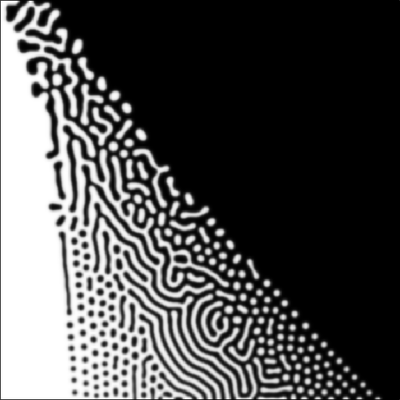
Without noise
Setting the parameter noise

u at time These mixed stripe-dot arrangements are expected to resolve very slowly (beyond the runtime of this movie).
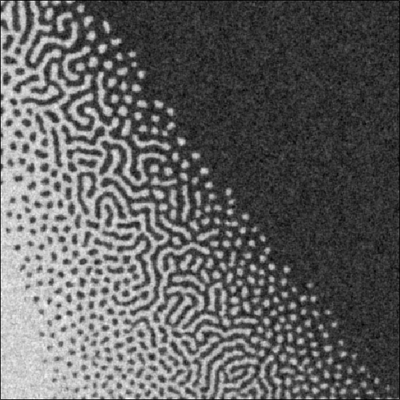
With noise
When adding little noise, then the above frustrated arrangements resolve faster (not shown).
With high noise level (noise
Moreover, continuously perturbing the fluxes keeps the state away from the homogeneous solution also in outside the Turing instability domain (towards the homogeneous white and black corners). There, the state relaxes back to the homogeneous state and gets pushed away again in a manner that the slowest-decaying spatial models dominate and are visible as apparent continuation of the Turing patterns (hexagonal array of dots) beyond the Turing instability border. These are known as noise-induced patterns.

u at time noise Reference
S. Miyazawa, M. Okamoto and S. Kondo: Blending of animal colour patterns by hybridization. Nature Communications 1: 66, 2010.
Model
model.xml
XML Preview
<MorpheusModel version="4">
    <Description>
        <Title>Example-TuringNoisy</Title>
        <Details>Extended model TuringPatterns (see https://morpheus.gitlab.io/model/m0014) by adding Gaussian noise to both PDEs. Solver was switched to Euler-Maruyama. We observe that the patterns emerge robustly under noisy conditions over the whole parameter plane (scanned by x- and y-dependent parameter values).

Also, continuously perturbed states outside the Turing instability domain try to relax back to the homogeneous state in a way that the slowest-decaying spatial models continue the Turing patterns (hexagonal array of dots) beyond the Turing instability border - known as noise-induced patterns.

The original (deterministic) model was published in:
Miyazawa, Okamoto and Kondo (2010). Blending of animal colour patterns by hybridization. Nature Communications 1, 66.
https://doi.org/10.1038/ncomms1071
</Details>
    </Description>
    <Global>
        <Field symbol="u" value="4.1+rand_uni(0,1)">
            <Diffusion rate="1"/>
        </Field>
        <Field symbol="v" value="4.84+rand_uni(0,1)">
            <Diffusion rate="20"/>
        </Field>
        <System time-step="0.25" name="Miyazawa" solver="Euler-Maruyama [stochastic, O(1)]">
            <Function symbol="A">
                <Expression>0.07 + ((0.07 * l.y)/ s.y)</Expression>
            </Function>
            <Constant symbol="B" value="0.08"/>
            <Function symbol="C">
                <Expression>-0.1 + ((0.5 * l.x)/ s.x)</Expression>
            </Function>
            <Constant symbol="D" value="0.03"/>
            <Constant symbol="E" value="0.10"/>
            <Constant symbol="F" value="0.12"/>
            <Constant symbol="G" value="0.06"/>
            <Constant symbol="R" value="20.0"/>
            <Constant symbol="synU_max" value="0.23"/>
            <Constant symbol="synV_max" value="0.50"/>
            <Function symbol="s_u">
                <Expression>max( 0, min( synU_max, A()*u-B*v+C()))</Expression>
            </Function>
            <Function symbol="s_v">
                <Expression>max( 0, min( synV_max, E*u - F))</Expression>
            </Function>
            <Constant symbol="noise" value="0.2"/>
            <DiffEqn symbol-ref="u">
                <Expression>R*(s_u() - D*u + rand_norm(0.0,noise))</Expression>
            </DiffEqn>
            <DiffEqn symbol-ref="v">
                <Expression>R*(s_v() - G*v + rand_norm(0.0,noise))</Expression>
            </DiffEqn>
        </System>
    </Global>
    <Space>
        <Lattice class="square">
            <Size symbol="s" value="512, 512, 0"/>
            <NodeLength value="1"/>
            <BoundaryConditions>
                <Condition type="noflux" boundary="x"/>
                <Condition type="noflux" boundary="y"/>
            </BoundaryConditions>
            <Neighborhood>
                <Order>1</Order>
            </Neighborhood>
        </Lattice>
        <SpaceSymbol symbol="l"/>
    </Space>
    <Time>
        <StartTime value="0"/>
        <StopTime value="100"/>
        <RandomSeed value="0"/>
        <TimeSymbol symbol="time"/>
    </Time>
    <Analysis>
        <Gnuplotter time-step="2" decorate="false">
            <Terminal name="png" persist="true"/>
            <Plot>
                <Field symbol-ref="u">
                    <ColorMap>
                        <Color color="black" value="1"/>
                        <Color color="white" value="0.0"/>
                    </ColorMap>
                </Field>
            </Plot>
        </Gnuplotter>
        <Logger time-step="0.0">
            <Input>
                <Symbol symbol-ref="u"/>
            </Input>
            <Output>
                <TextOutput file-format="csv"/>
            </Output>
            <Restriction>
                <Slice axis="x" value="s.x/2"/>
            </Restriction>
            <Plots>
                <Plot title="slice at half of x extension" time-step="-1">
                    <Style style="lines" line-width="3.0"/>
                    <Terminal terminal="png"/>
                    <X-axis>
                        <Symbol symbol-ref="l.y"/>
                    </X-axis>
                    <Y-axis>
                        <Symbol symbol-ref="u"/>
                    </Y-axis>
                    <Color-bar>
                        <Symbol symbol-ref="v"/>
                    </Color-bar>
                </Plot>
            </Plots>
        </Logger>
        <Logger time-step="2">
            <Input>
                <Symbol symbol-ref="u"/>
            </Input>
            <Output>
                <TextOutput file-format="csv"/>
            </Output>
            <Plots>
                <SurfacePlot time-step="2">
                    <Color-bar minimum="0" maximum="9">
                        <Symbol symbol-ref="u"/>
                    </Color-bar>
                    <Terminal terminal="png"/>
                </SurfacePlot>
            </Plots>
        </Logger>
        <ModelGraph include-tags="#untagged" format="svg" reduced="false"/>
    </Analysis>
</MorpheusModel>

Downloads
Files associated with this model: