
Reproducible cell surface mechanics
Parametrization
In CPM models the cell surface mechanics is determined by the interaction energies and the cell shape constraints. Contact and surface lengths are estimated from the cell representation in the lattice using neighborhood kernels, that are usually factored into the parametrization of the CPM’s surface mechanics. Since different CPM simulators have their particular choices for neighborhood kernels, rescaling of parameters may be required to reproduce published models among simulators. Of course, changing from a square to a hexagonal lattice or neighborhood sizes would require rescaling even within the same simulator.
Couldn’t one just normalize the parameters to the lattice node length to get rid of that issue? Well, in 2015 Magno et al. published a parameter normalization following the formalism of continuous surface mechanics (CSM). Every parameter of such a CSM parametrization can be transferred into a traditional CPM parameter using a neighborhood-specific correction factor ξ. Hence, also any CPM parametrization can be transferred to any other one using two ξ.
Conversion
With this blog we want to provide a resource to allow transfer of models between common CPM simulators. All notion is adapted to 2 dimensional models, but is as well valid for 3 dimensions. It is essential to know the exact neighborhood kernel choice of the simulators:
- Perimeter length : first order
- Interaction : user choice
- Perimeter length : 2nd order
- Interaction : 2nd order
Morpheus for a long time provides free neighborhood choice and both parametrizations under /CPM/ShapeSurface/@scaling :
- Normalized mode ‘norm’, using CSM parameters,
- Non-normalized mode ‘none’, using kernel-specific CPM parameters,
- A ‘classic’ mode is available since Morpheus 2.3.4, corresponding to the neighborhood choices of CC3D and the models by Glazier / Graner.
Normalized CSM parameters can be obtained from kernel-specific CPM parameters using these equations (see also 31a-c, Magno et al.):
Corresponding correction factors ξ for common neighborhood orders:
| order | square | hexagon | cubic |
|---|---|---|---|
| 1 | 1 | 2.2 | 1 |
| 2 | 3 | 6 | 5 |
| 3 | 5 | 10.4 | 9 |
| 4 | 11 | 22 | 11 |
| 5 | 15 | 28.6 | 23 |
| 6 | 18 | 36.2 | 39 |
| 7 | 26 | 52 | 47 |
| 8 | 36 | 69.1 | 70 |
And the derived CPM parameter conversion equations look as follows (also see Table 5, Magno et al.):
Note that switching hexagonal and square lattices requires to rescale the number of nodes, since the area of a hexagonal node is only
Results
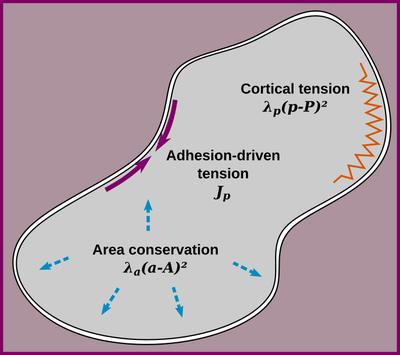
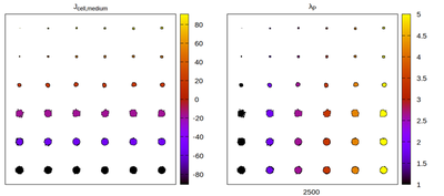
Let’s do a little exercise. The parameter plane model simulates an array of isolated cells, initialized with it’s target volume and simulated until a quasi steady state is reached. Cell properties
With
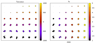
Panels differ by color coding
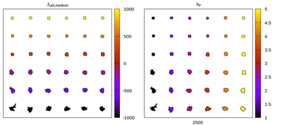
Now we convert the parameter set to kernel-specific CPM parameters and visually compare the results for different neighborhood choices. The rescaling works satisfactory, but for certain neighborhood choices artifacts appear.
Panels differ by color coding
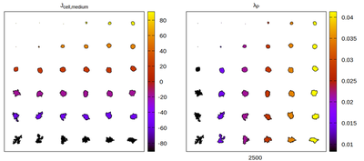
The Artistoo neighborhood choice
Panels differ by color coding
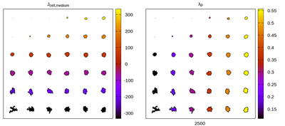
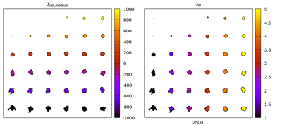
The CC3D neighborhood choice
The 1st order neighborhood
Panels differ by color coding
The hexagonal lattice
Finally, also switching to an hexagonal lattice can be performed the same way, but the target volume has to be rescaled in Morpheus by
Panels differ by color coding
In a follow up blog post we will study the emerging lattice artifacts in more detail.
References
Magno, R., Grieneisen, V.A. & Marée, A.F. The biophysical nature of cells: potential cell behaviours revealed by analytical and computational studies of cell surface mechanics. BMC Biophys 8, 8 (2015).